Point Cloud Density Splatter
 Punto de Ancla



Installation
PCD Splatter is a Blender extension, so installation is drag and drop.
Drag and drop — recommended
- Download
PCD_Splatter_v1.xx.x.zipfrom your Superhive receipt page. - Drag the
.zipfile into any Blender window. - Confirm the install dialog.
- The panel appears in the 3D Viewport sidebar. Press N and choose the PCD Splatter tab.
You can also install from your receipt page with one click, or through Edit ▸ Preferences ▸ Get Extensions ▸ Install from Disk.
Alternative — classic add-on method
Edit ▸ Preferences ▸ Add-ons ▸ Install from Disk- Select the
.zip— do not unzip it first. - Tick the checkbox next to Pointcloud Density Splatter.
- Press N in the 3D Viewport and choose the PCD Splatter tab.
Updating
Delete the previous version in Preferences ▸ Add-ons before installing a new one, then restart Blender. The version number is shown at the top right of the panel — check it after installing to confirm the new code loaded.
Requirements
- Blender 4.2 or newer (tested up to 5.1)
- Windows, macOS or Linux
-
No Python dependencies. Nothing to
pip install.
Quick start
The whole workflow is three steps:
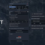
1. Inspect — Section Import, pick your file, press Inspect file. You get the exact point count, which fields the file carries, and the estimated memory.
2. Choose how much to load — Use the 1 % / 5 % / 10 % / 25 % shortcuts or type an exact number. The panel shows the estimated memory and warns you if it will not fit. Leave Split into tiles and Levels of detail on for anything above a couple of million points.
3. Create — Press Create splat object. A progress bar shows each stage and can be cancelled.
Then navigate. The object is created in navigation mode, which means the node tree contains no reference to the camera, so moving the view does not recompute anything. When you are ready to render, press Prepare for render in the Detail section.
Documentation
Section 1 — Import
| Control | What it does |
|---|---|
| Point cloud | PLY, E57, PTS, XYZ, ASC, TXT or CSV |
| Inspect file | Reads only the header. Instant even on multi-GB files |
| Axes | Leave at No change for E57, which is already Z-up |
| Limit the import | Reads only part of the cloud, decimating while reading |
| Points to import | Takes 1 in every N spread across the whole file |
| Split into tiles | Splits the cloud into spatial tiles, each its own object |
| Points per tile | Smaller tiles allow finer culling; many objects have a cost |
| Levels of detail | Builds merged versions of each tile |
Section 2 — Conversion
These are baked into the mesh: changing them requires rebuilding.
Shape and orientation. Splat shape picks between Surfel (oriented by the surface normal — classic surface splatting, best on scans), Billboard (always faces the camera) and Round (unoriented, useful for vegetation or dust). Estimate normals fills them in for files that carry none, which is most E57 and PTS files. Smooth orientation interpolates between neighbouring cells — leave it on, or a visible lattice appears.
Density. Measure point spacing computes the real distance to each point's neighbour. Smooth density averages it; without this, splat size varies randomly point to point and produces mottling at high Coverage.
Reduction. Voxel decimation, Morton ordering and a hard cap on splats.
Initial values. Blend mode, single-sided, splat size, visible points, adaptive and anisotropy — the state the object starts in.
Section 3 — Size
Adaptive blends between one uniform size and per-point sizing from the measured spacing. Coverage multiplies that measured spacing. Anisotropy stretches splats along each surface's dominant direction. All live: no rebuild needed.
Section 4 — Appearance
Six display modes, two blend modes and the shader gains.
Dithered writes to the Z-buffer, so occlusion is always correct. It looks grainy while you navigate and resolves when you stop. Blended gives a smooth gradient from the first frame but does not write depth, so a distant splat can cover a near one — enable Depth sort to fix that, at the cost of re-evaluating when the camera moves.
Single sided draws each card only on its front face, like a game engine's backface culling. It deletes no points.
If you are using Cycles, this section will warn you about black edges and offer a one-click fix. See the FAQ.
Section 5 — Culling
Chained cheapest to most expensive: point budget and distance, then section plane, frustum, backface, and the geometry mask last.
Section plane is the standout tool for industrial work: press Create clip plane, then move and rotate the Empty to cut into the scan live.
Assigning an object to any of these sockets uses the Refresh button at the top of the section if the change does not appear — Blender does not always rebuild its dependency graph when a socket gains a new object.
Section 6 — Detail
Two lists — levels and tiles — with the splat count of each, which one is being drawn and which one is being edited. A fixed row at the top switches level with one click. Apply to the whole set pushes one setting to every tile and level at once.
Draw distance controls the view radius, the target on-screen detail and the settle delay. Preview mode shows a light level in the viewport while the render uses full resolution — this is what makes camera animation smooth. Prepare for render turns everything back on before F12.
Section 7 — Performance
Visible point budget with percentage shortcuts and a refresh button. Navigation mode swaps to a node tree with no camera reference at all. Realize instances turns each splat into real geometry — needed to apply the modifier or export to other formats, not to render.
Section 8 — Export
From the scene writes what you are actually looking at: tiles, decimation and settings already applied. From the original file re-reads the source and applies only this panel's values.
 Included
Includes 12 months of
- Support from Punto de Ancla
- Product updates
Extend this product’s Support Period +12 months: 50% of product price
Have questions before purchasing?
Login to message
| Blender Extension Compatible | Yes |
| Published | about 2 months ago |
| Blender Version | 4.2 - 5.2 |
| Extension Type | Add-on |
| Render Engine Used | Cycles, Eevee |
| License | GPL |
Discover more products like this
point cloud addon 3D Gaussian Splatting conversion geometrynodes Gaussian Splat ply e57 3d gaussian splats pts gaussian splatting point cloud