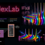
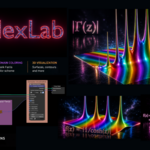
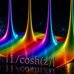
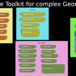
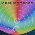
ComplexLab is a Geometry Nodes toolkit designed to create, combine, and visualize complex-valued functions directly in Blender. It provides a modular node-based workflow for transforming the complex plane into customizable 3D surfaces, topographic maps, and colorful mathematical patterns.

The different nodes are organized into four categories:

1) Graph

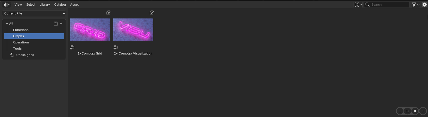
• Complex Grid: Generates the mesh representing the complex plane.
  
• Complex Visualization: Turns a complex-valued function into a customizable 3D visualization. Use simple checkboxes to display the real part, imaginary part, modulus, iso-modulus (topographic) lines, and other visualization layers independently or in combination.
  
  

2) Operations :

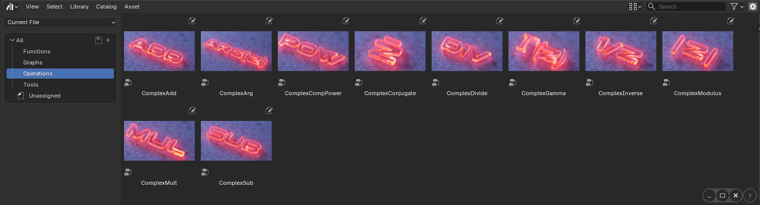
The Operations submenu provides nodes for performing mathematical operations on complex values. That includes :

• addition
• subtraction
• multiplication
• division
• powers
• conjugate
• inversion
• modulus
• argument

These nodes can be combined to build custom complex expressions and more advanced function networks.

3) Tools :

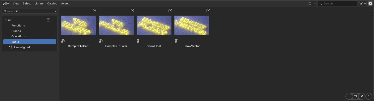
The Tools submenu provides utility nodes :

• ComplexToCart : Converts a complex value into its Cartesian representation using its real and imaginary components.
• ComplexToPolar : Converts a complex value into its polar representation using its modulus and argument.
• ShowFloat : Displays a single numerical value directly in the node interface.
• ShowVector : Displays a vector value directly in the node interface.

4) Functions :

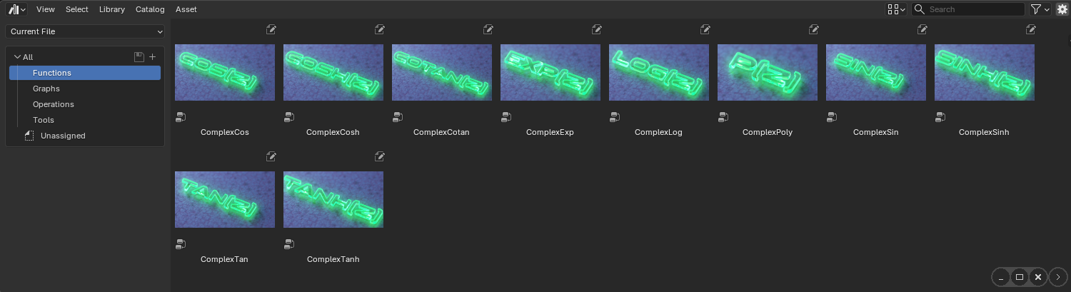
The Functions submenu provides nodes for applying common complex-valued functions:

• Cos: Computes the complex cosine of the input value.
• Sin: Computes the complex sine of the input value.
• Tan: Computes the complex tangent of the input value.
• Cosh: Computes the complex hyperbolic cosine.
• Sinh: Computes the complex hyperbolic sine.
• Tanh: Computes the complex hyperbolic tangent.
• Exp: Computes the complex exponential.
• Log: Computes the complex logarithm.
• Polynomial: Creates a customizable polynomial function.
• Gamma: Computes the complex Gamma function.

Usage Workflow

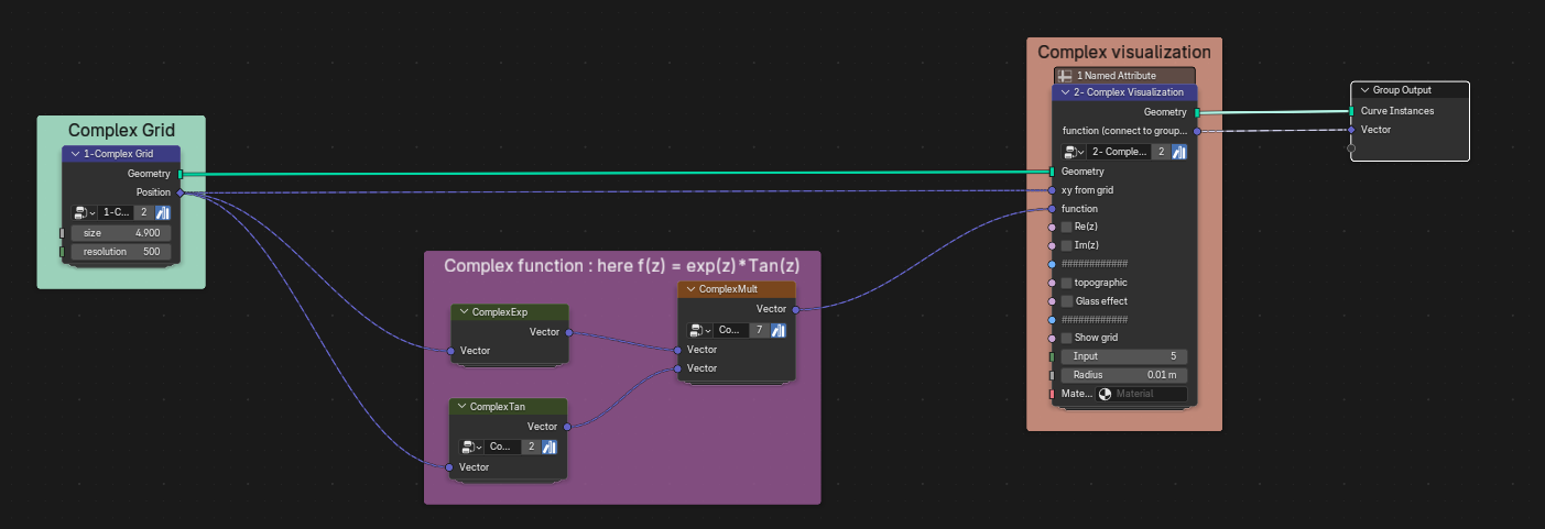
The workflow begins with the Complex Grid node, which generates complex coordinates $z\; =\; a\; +\; ib$. These coordinates are then connected to one or more function and operation nodes. In the example below, they are used to define $f(z)=\exp (z)\tan (z)$. The resulting complex function is sent to the Complex Visualization node, where its appearance and display options can be adjusted before generating the final geometry.

Below is a short video demonstrating how to use the nodes.

Nota Bene - Representing a Complex Function

A complex-valued function f : ℂ → ℂ requires four real dimensions to be represented completely.

The input is a complex number z = x + iy, described by two real coordinates:x = Re(z) and y = Im(z).

The output is also complex: f(z) = u(x,y) + iv(x,y), and therefore requires two additional real coordinates: u = Re(f(z)) and v = Im(f(z)).

A complete representation would therefore require four coordinates(x, y, u, v), corresponding to an object in four-dimensional real space ℝ⁴.

ComplexLab uses color to encode the fourth dimension. The real and imaginary parts of the input, Re(z) and Im(z), define the horizontal plane, while the modulus |f(z)| determines the height of the surface. The argument arg(f(z)) is represented through color.

The color mapping used in ComplexLab follows the complex-function visualization scheme described by Frank A. Farris, in which the argument of a complex value is associated with a color. This approach makes it possible to visualize both the magnitude and phase of a complex function within a three-dimensional representation.

Reference: Frank A. Farris, Domain Coloring and the Argument Principle